Smooth Mesh Gradients with RBF Interpolation

Author: Pavel Kolesnikov (linkedin, website)

Try the implementation on web or figma

1. Introduction

Mesh gradients are a powerful way to create smooth, organic color transitions. Traditional techniques like spline-based interpolation or multiple overlapping radial gradients can be effective—but they also come with trade-offs: visual artifacts, complexity, or the need for structured meshes.

In this article, I’ll show you how to use Radial Basis Function (RBF) interpolation to generate seamless gradients from just a set of colored points. This approach is portable, flexible, and simple to implement.

2. Intuition Behind RBFs

Imagine placing a glowing colored dot on a canvas. The closer you are to the center of that dot, the more intense the color. When you place multiple such dots, the colors blend together based on proximity.

This is the essence of Radial Basis Functions. Each point emits a smooth influence that fades with distance. By summing the influence of all points, we get a continuous gradient across the entire surface.

3. Mathematical Foundation

a. Problem Definition

Let’s say we have $N$ points $(x_1, y_1), (x_2, y_2), \ldots, (x_N, y_N)$ each with a corresponding color $c_1, c_2, \ldots, c_N$ . We want to find a function:

f(x, y) \rightarrow \text{color}

that satisfies the constraint:

f(x_i, y_i) = c_i \quad \text{for all } i

and produces smooth color transitions in between.

b. The RBF Function

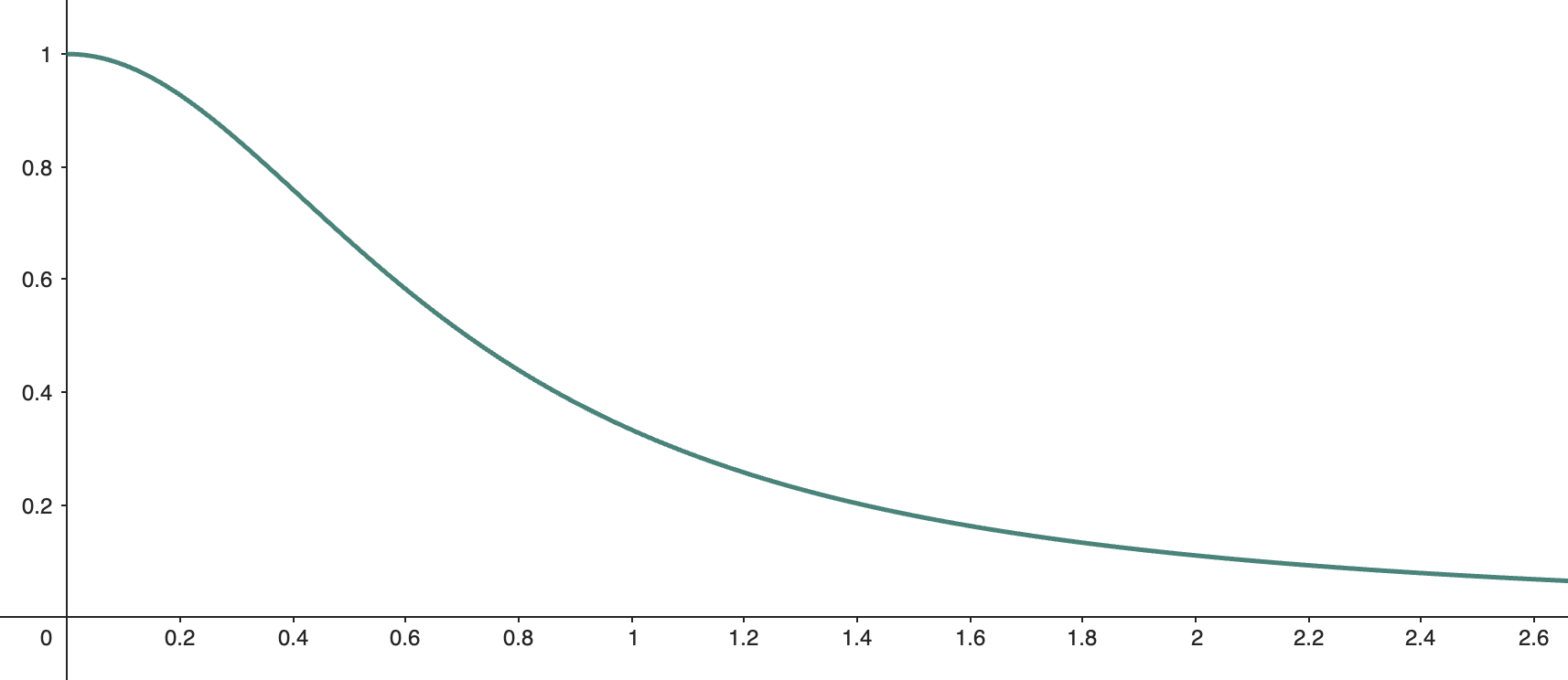
We define an RBF as a function that depends only on the distance between two points. One form that works well in practice is:

\text{RBF}(x_0, y_0, x_1, y_1) = \frac{0.5}{(x_0 - x_1)^2 + (y_0 - y_1)^2 + 0.5}

You can also express this in terms of a radial distance $r$ : $\text{RBF}(r) = \frac{0.5}{r^2 + 0.5}$

This function has two nice properties:

It peaks at 1 when $r = 0$ , and approaches 0 as $r$ increases.

It's smooth and almost flat near the center, ensuring continuity.

Here's what the RBF curve looks like (X-axis is $r$ ):

c. The Interpolated Function

We define our color function as a weighted sum of RBFs centered at each control point:

$f(x, y) = \sum_{i = 1}^N a_i \cdot \text{RBF}(x, y, x_i, y_i)$

Here, the weights $a_i$ are what we need to solve for.

4. Solving for Coefficients

To determine the weights $a_i$ , we enforce the condition:

f(x_i, y_i) = c_i

Substituting our definition of ff into each constraint gives us a system of linear equations:

\begin{aligned} a_1 \cdot \text{RBF}(p_1, p_1) + a_2 \cdot \text{RBF}(p_1, p_2) + \ldots + a_N \cdot \text{RBF}(p_1, p_N) &= c_1 \\ a_1 \cdot \text{RBF}(p_2, p_1) + a_2 \cdot \text{RBF}(p_2, p_2) + \ldots + a_N \cdot \text{RBF}(p_2, p_N) &= c_2 \\ &\vdots \\ a_1 \cdot \text{RBF}(p_N, p_1) + a_2 \cdot \text{RBF}(p_N, p_2) + \ldots + a_N \cdot \text{RBF}(p_N, p_N) &= c_N \end{aligned}

In matrix form:

\begin{bmatrix} \text{RBF}(p_1, p_1) & \cdots & \text{RBF}(p_1, p_N) \\ \vdots & \ddots & \vdots \\ \text{RBF}(p_N, p_1) & \cdots & \text{RBF}(p_N, p_N) \end{bmatrix} \begin{pmatrix} a_1 \\ a_2 \\ \vdots \\ a_N \end{pmatrix} = \begin{pmatrix} c_1 \\ c_2 \\ \vdots \\ c_N \end{pmatrix}

This is a standard system of linear equations. Once you've computed the RBF matrix, you can solve it using any linear algebra library or by implementing some of the algorithms on your own (not recommended).

5. Implementation

The implementation closely follows the algorithm above, with a few practical additions for graphics use.

a. Input Interface

I built a simple UI to interactively create and manipulate control points: adding, dragging, and assigning colors. Internally, it’s represented as an array of colored points:

[
  {
    "x": 0.3,
    "y": 0.5,
    "color": [255, 0, 0]
  },
  {
    "x": 0.7,
    "y": 0.2,
    "color": [0, 0, 255]
  }
]

Each point has normalized coordinates and an RGB color.

b. Computing the Weights

Since colors are vectors (RGB), we solve for three separate weight sets: red, green, and blue.

Build the RBF matrix (same for all channels):

function rbf(p1, p2) {
  const r2 = (p1.x - p2.x) ** 2 + (p1.y - p2.y) ** 2;
  return 0.5 / (r2 + 0.5);
}

const matrix = points.map(p1 => points.map(p2 => rbf(p1, p2)));

Invert the matrix using a linear algebra library.

const inverseMatrix = invert(matrix); // Use your favorite lib

Multiply the inverse matrix with each color component vector:

const redWeights = multiply(inverseMatrix, points.map(p => p.color[0]));
const greenWeights = multiply(inverseMatrix, points.map(p => p.color[1]));
const blueWeights = multiply(inverseMatrix, points.map(p => p.color[2]));

c. Rendering with WebGL

Rather than compute each pixel in JavaScript, we offload interpolation to the GPU via a fragment shader.

Vertex shader:

in vec4 position;
void main() {
  gl_Position = position;
}

Fragment shader:

uniform vec2 points[100];
uniform vec3 weights[100];

float rbf(vec2 p1, vec2 p2) {
  float d = distance(p1, p2);
  return 0.5 / (0.5 + d * d);
}

vec3 interpolate(vec2 point) {
  vec3 color = vec3(0.0);
  for (int i = 0; i < 100; i++) {
    color += weights[i] * rbf(points[i], point);
  }
  return color / 255.0;
}

void main() {
  vec2 uv = gl_FragCoord.xy / resolution.xy;
  uv.y = 1.0 - uv.y;
  vec3 c = interpolate(uv);
  gl_FragColor = vec4(c, 1.0);
}

Just compile your shaders, pass uniforms, and enjoy smooth GPU-powered gradients 🎉

6. Final Thoughts

There are still interesting directions to explore:

Animating: The described process can be very quick. If you have a small amount of points, you can programmatically animate their coordinates and colors and perform the same algorithm on each update, it’ll generate animated gradients.

Tuning the RBF: The falloff function can be adapted for different resolutions and aesthetic goals. Making it parameterized and optimizing it could lead to even smoother results.

Regularization: Adding a regularization term when solving for weights may help reduce artifacts or overshooting near dense clusters.

Whether you're building a design tool, a shader playground, or just exploring beautiful math in graphics—this method is flexible, elegant, and performant.

Happy rendering! 🙂